Most methods used for data analysis for spectra from metabonomic studies base on the family of data decomposition methods. The most prominent members are the unsupervised principal component analysis (PCA) and the supervised partial least squares (PLS) methods. The principles of PCA are briefly illustrated.
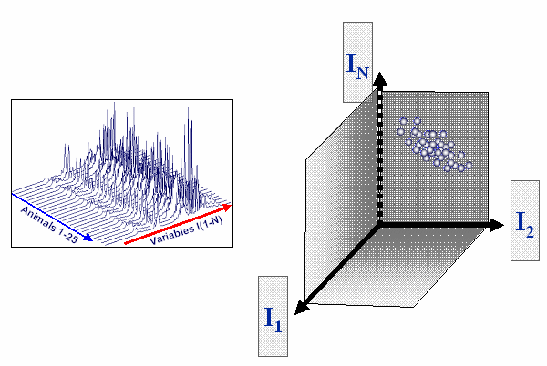
A sample represented by a spectrum with only 3 variable can be seen as a point (or vector beginning a the origin of the coordinate system) in the 3-dimensional space, which is spanned by the three variables. The values of the 3 variables determine the location in space.
A sample with a spectrum containing only 3 variables can be seen as a point spanned in the 3-dimensional space of the 3 variables.
In the case of a metabonomic study, typically not only 3 but n variables are measured. Also not only 1 sample but several samples are investigated. In that case the space is not 3-dimensional but n-dimensional, which cannot be visualized in graphical way anymore. The samples form a cloud in the n-dimensional space. PCA is used to reduce the n dimensions to a number, which can be easily visualized.
Typcial situation in the case of a metabonomic study with n spectral variables forming a n-dimensional space and several samples forming a cloud of points.
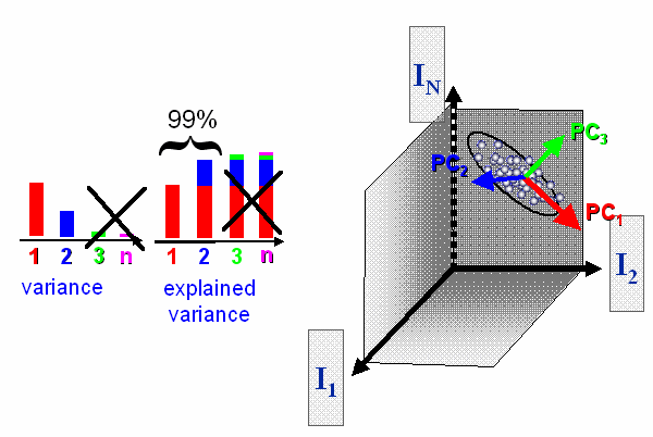
The PCA looks for a new coordinate system, which is optimal for reducing the number of dimensions. The first new coordinate axis, which is also called principal component 1, is the direction in space, for which the samples have the highest variance. The second coordinate is the direction in space orthogonal to principal component 1, which explains most of the remaining variance. This procedure is repeated until n new principal components are formed. The most important property of the new coordinates is decrease of variance explained per component. Therefore only few principal components explain the majority of the variance. It is assumed that the variance of the higher principal components only contains noise. Therefore the higher components can be skipped and the problem is reduced to a lower number of dimensions.
The PCA looks for a new orthogonal coordinate system, which explains most of the variance by the first few coordinates.
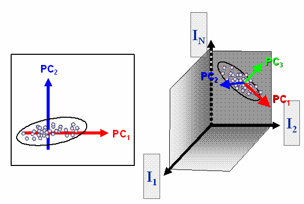
The PCA allows capturing the information in a low number of principal components. Therefore an easy analysis and visualization of the data is possible. In contrast to PCA, PLS uses information about a dependent variable (concentration, membership to classes...) to find a new coordinate system for the independent variables, not only explaining most of the variance, but also is predictive for the dependent variable (covariance).
The low number of most important coordinates allows an easy analysis and visualization of the data.